Theory of Computation Notes
— 22 min read
Table of Contents
Introduction
These are my notes on theory of computation.
Mathematical Notions and Terminology
This section covers the fundamental building blocks.
Sets
A set is a group of objects. It can contain any type of object like numbers, symbols, and other sets. The objects in a set are called elements or members. In a set, the ordering of elements and repetition doesn't matter.
For example:
Definitions
- and means membership and nonmembership
- and
- is read as is a subset of . It means that all elements of is also in .
- is read as is a proper subset of . It means that all elements of is also in , BUT is not exactly the same as , that is, has fewer elements.
- describes a set containing elements according to a rule.
- describes the union of two sets and , combining all elements from both into a single set.
- describes the intersection of two sets and , containing only the elements common to both.
- is the complement of A, containing all elements not in .
- is the power set of , containing all possible subsets of , including the empty set and itself.
- is the Cartesian product or cross product of and , is the set containing all ordered pairs where the first element and the second element . Read as cross .
- Cartesian products can involve more than just pairs:
- is a Cartesian product of a set with itself.
Examples
- Natural numbers: = {1, 2, 3, ...}
- Integers: = {..., -2, -1, 0, 1, 2, ...}
- Empty set:
- Singleton set: a set with one element, e.g.,
- Unordered pair: a set with two elements, e.g.,
- : the set of perfect squares
- If , then .
- is the set of all ordered pairs whose elements are 0s and 1s.
- Let and
Sequences and Tuples
A sequence is a list of objects in some order designated with parentheses. In sequences, order and repetition matters.
For example:
However:
- Finite sequences are called tuples.
- A -tuple is a sequence with elements. is a 3-tuple.
- A 2-tuple is called an ordered pair.
Functions and Relations
A function is a thing that takes an input and produces and output. Similarly, given , is a mapping, that is, maps to . The same input always yields the same output.
- Domain: the set of all possible inputs of a function
- Range: the set of all possible outputs of a function, also called the codomain
- Given a domain and a range , , is read as maps to . This is called a function notation or mapping notation. Writing this function notation is also said to be "defining the codomain".
- A function is onto or surjective if all elements in the output set is matched or mapped by at least one element from the input set . This means the function reaches every possible output. The codomain must be defined in order to determine if a function is onto or not.
- A binary relation R is reflexive if for every ,
- A binary relation R is symmetric if for every and , implies
- A binary relation R is transitive if for every , , and , and implies
- A binary relation R is an equivalence relation if is reflexive, symmetric, AND transitive.
Examples
- defined by is onto.
- defined by is NOT onto.
Graphs
- An undirected graph or graph is a set of points with lines connecting (or not) the points.
- The points are referred to as vertices or nodes.
- The lines are called edges.
- The degree of a node refers to the number of edges at that node.
- A self-loop is an edge from a node to itself.
- Given a graph containing nodes and , the pair represents the edge connecting and . The order of the pair doesn't matter in an undirected graph, i.e., and is the same edge. Another way to describe these undirected edges with unordered pairs is with set notation:
- Given a graph , being the set of nodes of , and being the set of edges of , . This can be used to formally describe graphs.
- A labeled graph is a graph with labels on nodes and/or edges.
- Given a graph , a graph is considered to be a subgraph of if is formed by a subset of the vertices and edges of .
- A path is a sequence of nodes connected by edges in a graph.
- A simple path is a path that doesn't repeat any nodes.
- A graph is connected if every two nodes in that graph have a path between them.
- A cycle is a path that starts and ends at the same vertex.
- A simple cycle is one that contains at least three nodes and repeats only the first and last nodes.
- A tree is a graph that is connected and has no simple cycles.
- The leaves of a tree are nodes with a degree 1.
- A directed graph uses arrows instead of lines. This set of edges in directed graphs have ordered pairs.
- Outdegree refers to the number of arrows pointing out from a node.
- Indegree refers to the number of arrows pointing into a node.
- A directed path refers to a path in which all the arrows point in the same direction as it steps.
- A directed graph is strongly connected if a directed path connects every two nodes.
Strings and Languages
An alphabet is a nonempty finite set whose members are called symbols.
Examples of alphabets:
A string over an alphabet is a finite sequence of symbols from that alphabet. For example, given from above, then "01001" is a string over . Another example, given from above, "abracadabra" is a string over .
- is the length or number of symbols in the string over .
- A string of length zero is called the empty string denoted by . It plays the role of a 0 in a number system. For example: if , then . The here indicates string concatenation.
- If string has length , then where each . For example: then , , and .
- is the reverse of , i.e.,
- concatenates a string with itself times, e.g.,
- Lexicographic order is a way of ordering strings, e.g., a dictionary.
- Shortlex order or string order orders strings with shorter strings always coming first. E.g., the string ordering of all strings over the alphabet is .
- A string is considered to be a prefix of string if a string exists where . In other words, string is a prefix of another string if you can append some string to to get . E.g., let and , then .
- A string is a proper prefix of string if is a prefix of and . This means must be non-empty.
- A language is a set of strings formed from an alphabet.
- A prefix-free language is a language where no strings in the language is a proper prefix of any other string in the language. E.g., is NOT prefix-free because "a" is a proper prefix of both "ab" and "abc". But, is considered to be prefix-free.
Boolean Logic
Boolean logic is a mathematical system based on the values TRUE and FALSE represented as 1 and 0.
Boolean Operations
-
Negation (NOT): The operation that inverts a Boolean value.
-
Conjunction (AND): The operation that results in 1 if both operands are 1.
-
Disjunction (OR): The operation that results in 1 if at least one operand is 1.
-
Exclusive OR (XOR): The operation that results in 1 if one operand is 1 and the other is 0.
-
Equality (XNOR): The operation that results in 1 if both operands are the same.
-
Implication: The operation that results in 0 only if the first operand is 1 and the second is 0.
Boolean Identities
Boolean operations can be expressed in terms of AND and NOT:
Distributive Law
Boolean logic follows distributive laws similar to arithmetic:
Theory of Computation
There three are central areas of the theory of computation:
- Automata theory
- Computability theory
- Complexity theory
This question connects all three areas:
What are the fundamental capabilities and limitations of computers?
Automata Theory
Automata theory is about the definitions and properties of mathematical properties of computation.
DFA
DFA (deterministic finite automata) is a state machine with states (nodes) and transitions (edges) labeled with symbols.
DFA Formal Definition
A finite automata is a 5-tuple where:
- is a finite set of states
- is a finite alphabet
- is the transition function
- is the start state
- is the set of accepting states
If is the set of all strings that machine accepts, we say that is the language of machine and write . We say that recognizes or that accepts .
Formal Definition of Computation
A language is called a regular language if some finite automaton recognizes it.
Regular Operations
Let and be languages. We define regular operations union, concatenation, and star:
- Union:
- Concatenation:
- Star: , the empty string is always a member of no matter what is
NFA
NFA (non-deterministic finite automata) is a type of state machine where the machine may transition into multiple possible states from a given state and input symbol. It can also have transitions that occur without consuming any input called -transitions.
Differences Between DFA and NFA
- Every state of a DFA always has exactly one exiting transition arrow for each symbol in the alphabet.
- In an NFA, a state may have zero, one, or many exiting arrows for each alphabet symbol.
- NFAs can have -transitions. In particular, a state with only one transition, that being an -transition, can split into two copies, one that follows the exiting -transition and one staying at the current state.
NFA Formal Definition
Similar to DFA except the transition function takes a state and an input symbol or the empty string and produces the set of possible next states.
- is a finite set of states
- is a finite alphabet
- is the transition function
- is the start state
- is the set of accepting states
Union Operation Proof
There are two versions of this proof, one that doesn't use nondeterminism and one that does.
Deterministic Version
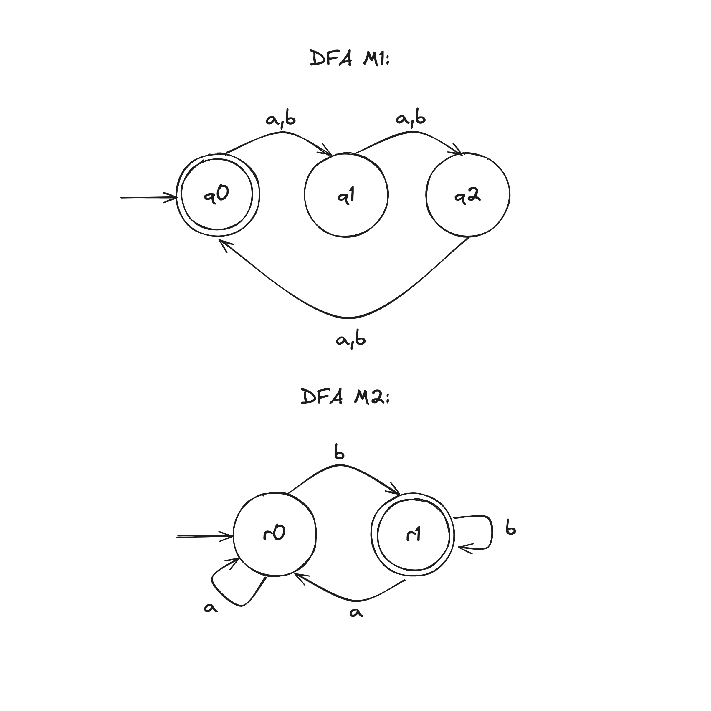
Let DFA recognize .
Let DFA recognize .
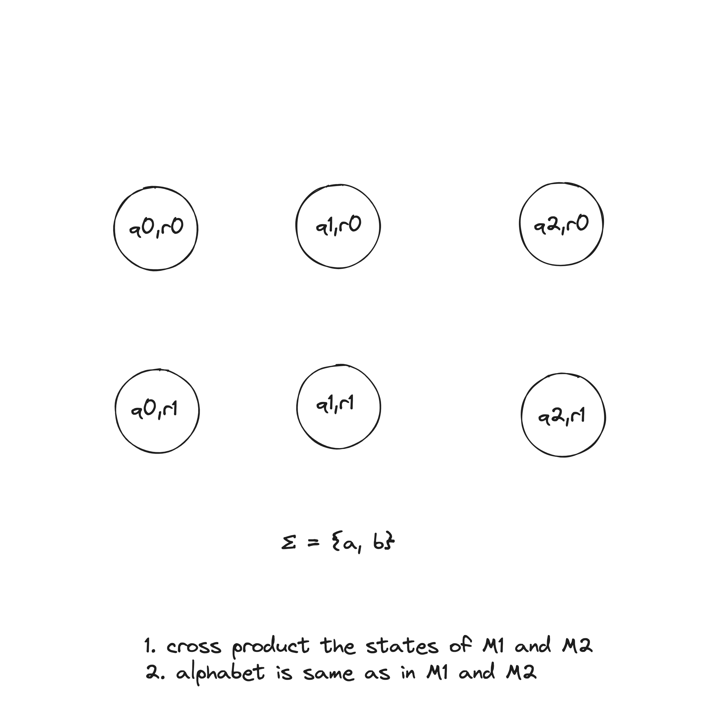
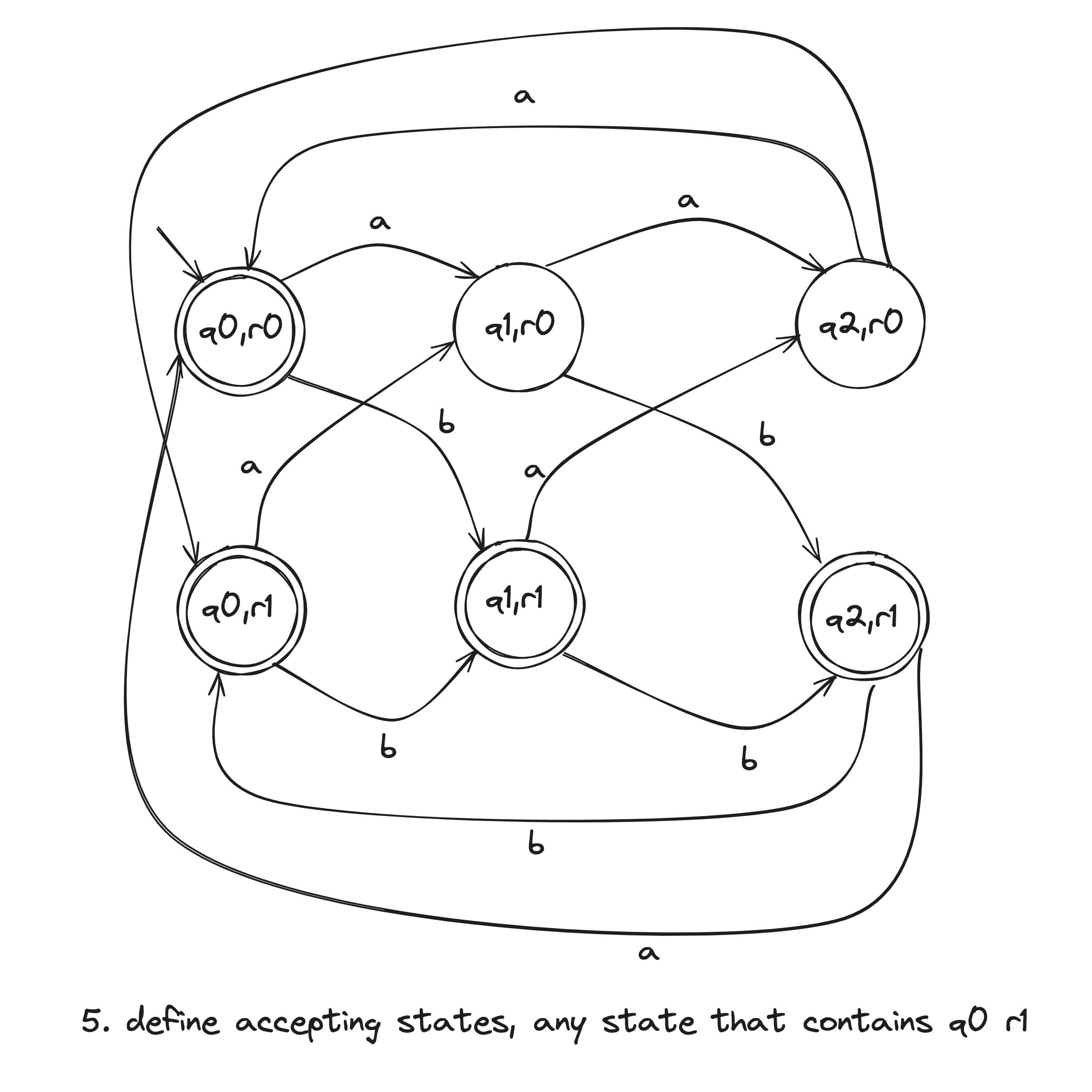
Construct DFA to recognize .
- . This set is the Cartesian product of sets and and is written . It is the set of all pairs of states, the first from and the second from .
- , the alphabet, is the same as in and .
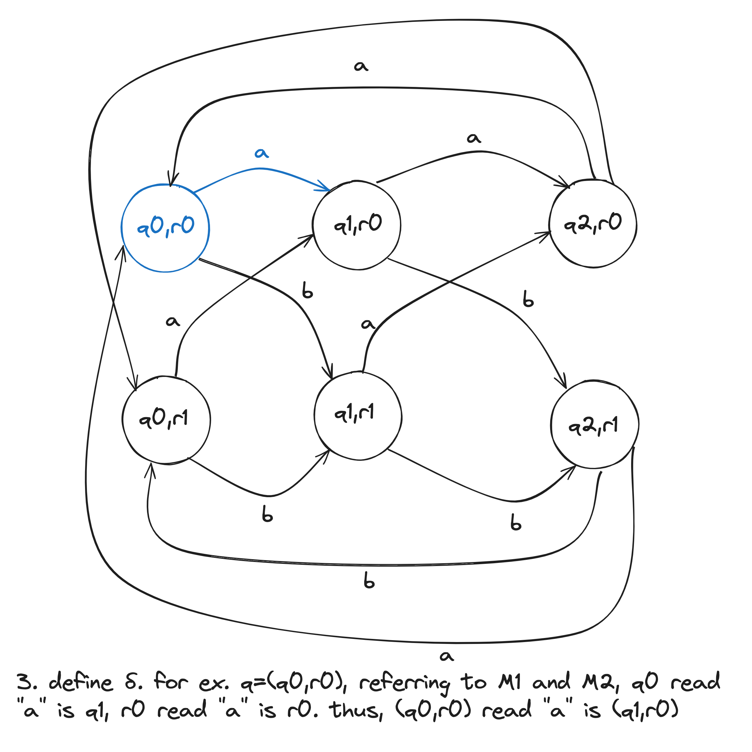
- For each and , let .
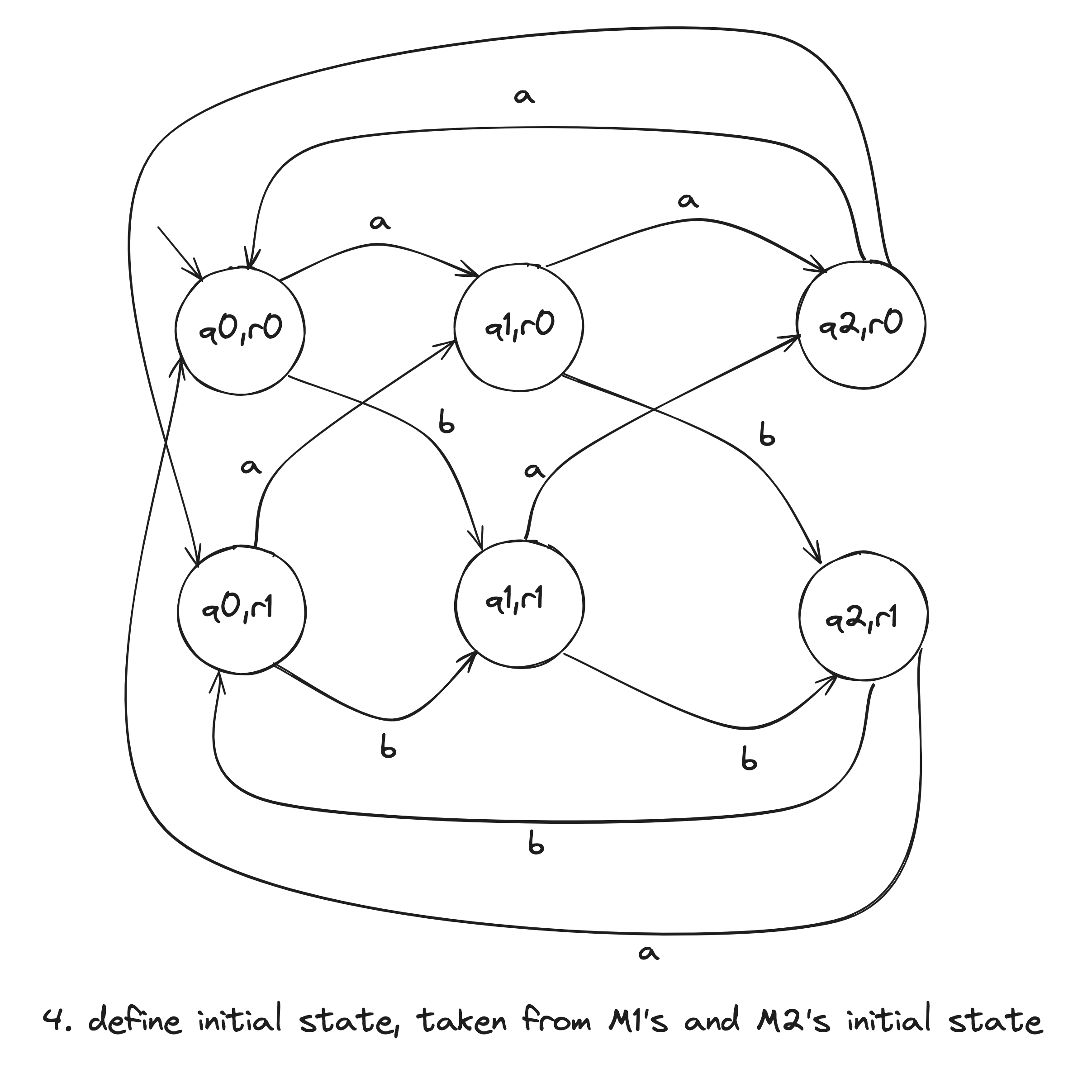
- is the pair .
- is the set of pairs in which either member is an accept state of or : . This can be also written as .
Nondeterministic Version
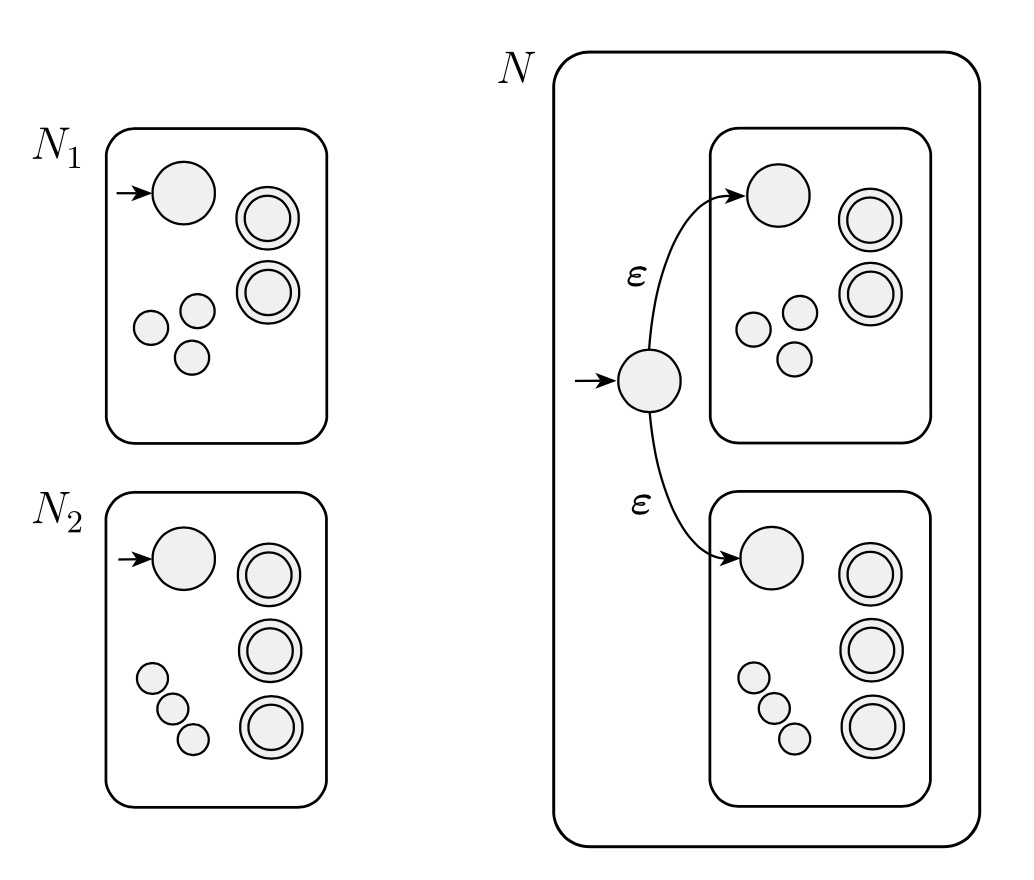
Let recognize .
Let recognize .
Construct NFA to recognize .
- is the new start state of
- Define so that for any and any :
Concatenation Operation Proof
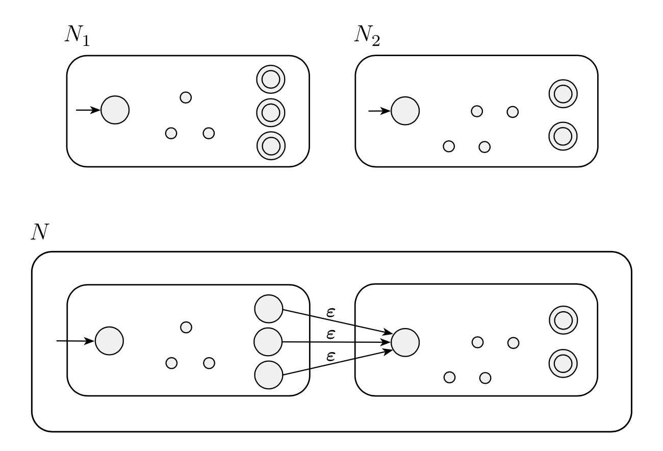
Let recognize .
Let recognize .
Construct NFA to recognize .
- Define so that for any and any :
Kleene Star Operation Proof
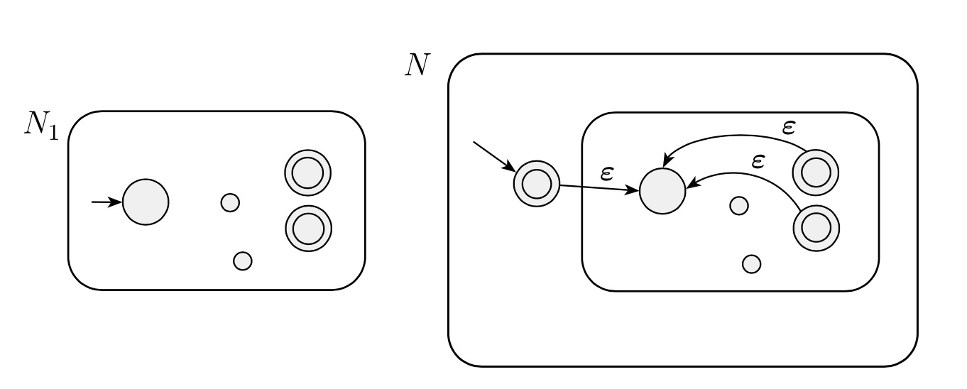
Let recognize .
Construct NFA to recognize .
- . The states of are also the states of plus a newly added state.
- The state (the newly added state) is the new start state.
- . The newly added state is then added to the set of old accept states.
- Define so that for any and any :
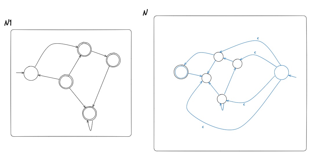
Reverse Operation Proof
Let that recognizes .
Construct NFA to recognize .
- is the new start state
- For any , if and
Perfect Shuffle Proof
Let recognize .
Let recognize .
Let
Construct DFA to recognize .
- Define so that for any , any , and any :
NFA to DFA
Given an NFA, there is an equivalent DFA.
Let NFA recognize .
Construct DFA to recognize .
Assuming No Epsilon Transitions
- , note that where is the size of
- For and ,
Assuming Epsilon Transitions
i am lost, this proof omg
NFA to DFA Example
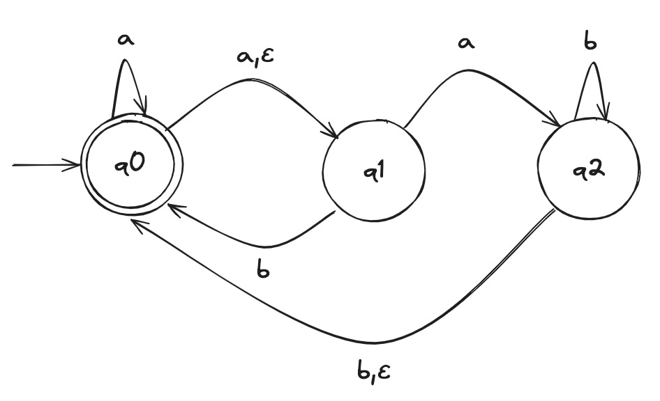
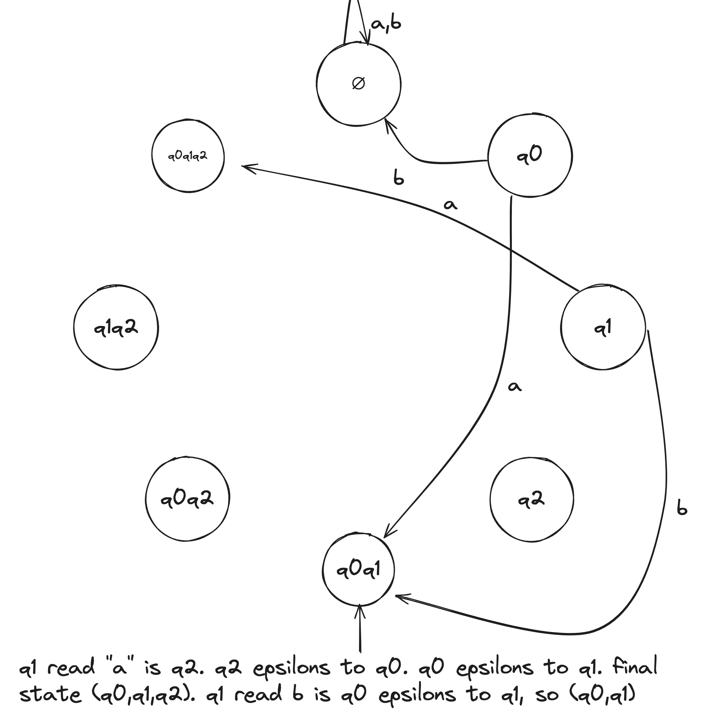
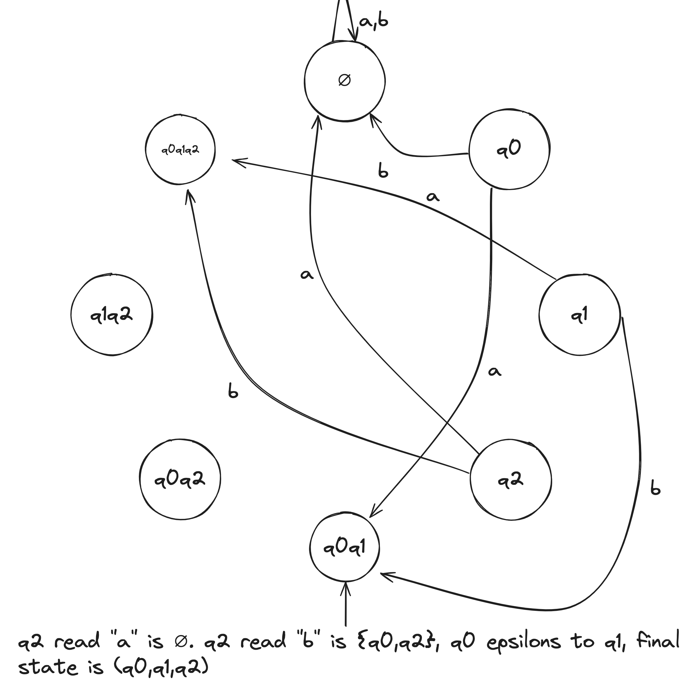
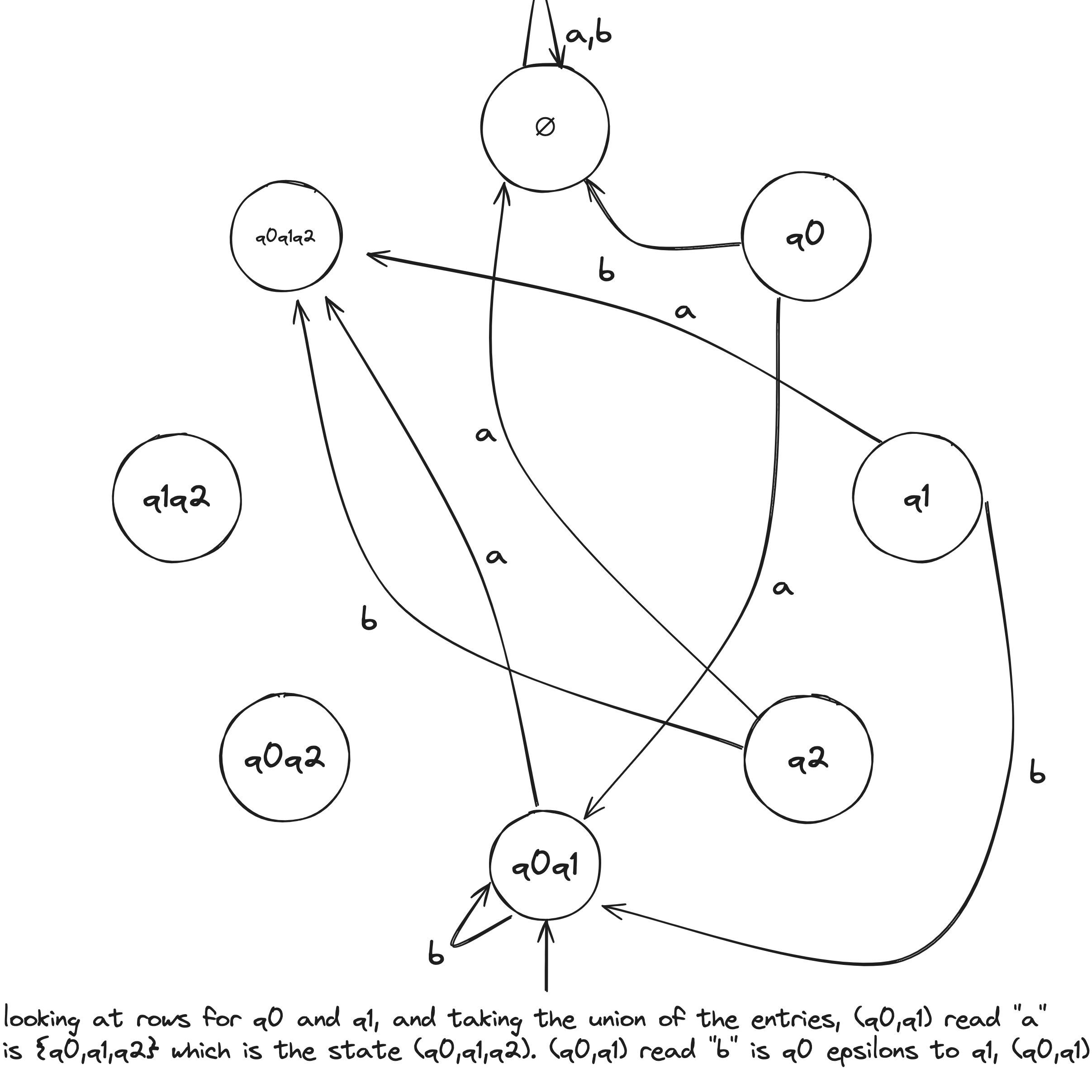
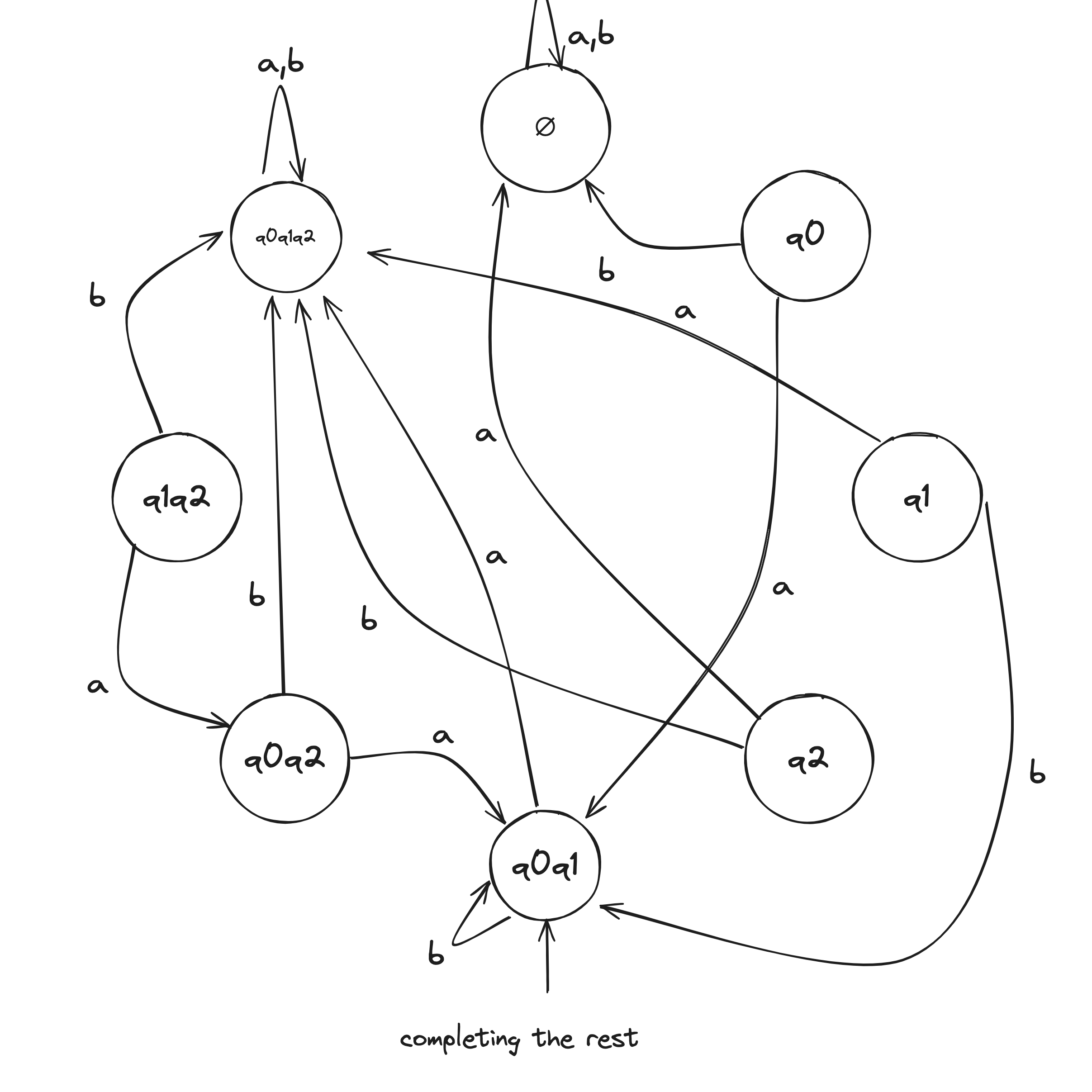
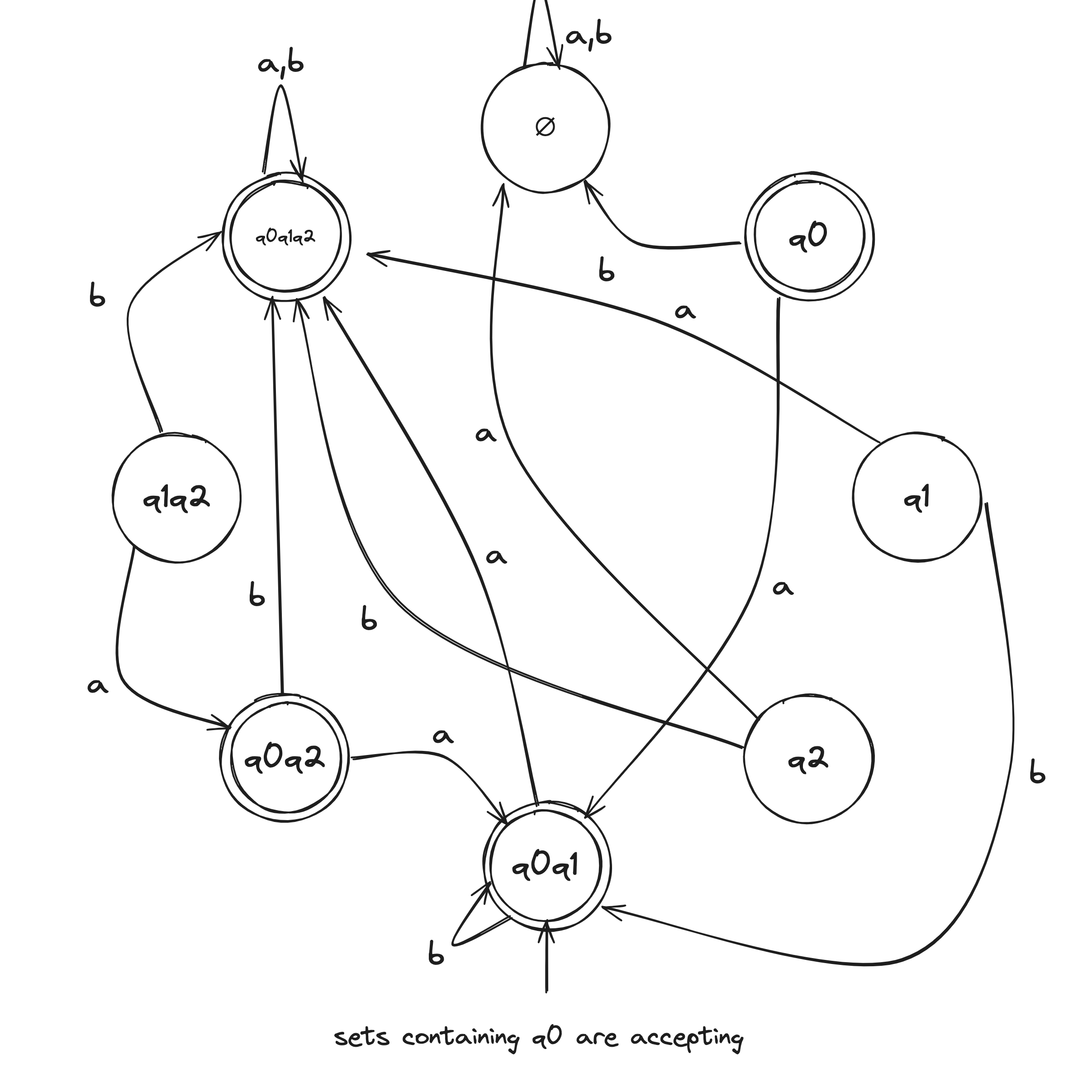
Given the above example NFA ( is implicitly in the language), we construct a DFA in the following:
- Build NFA table.
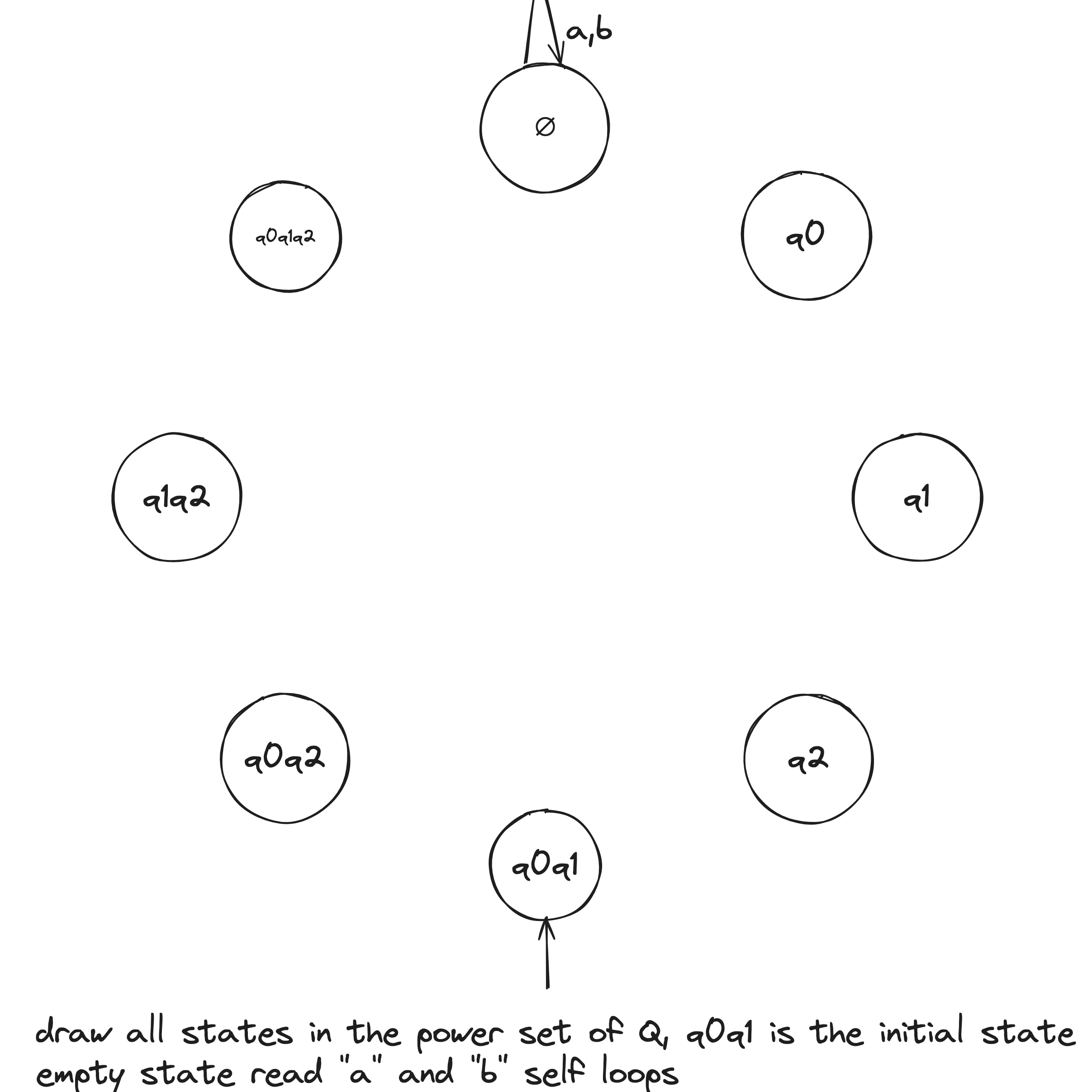
- Define initial state to be the states reachable from on epsilon transitions: .
- Draw with initial state . And, the state self loops when reading any symbol in the alphabet.
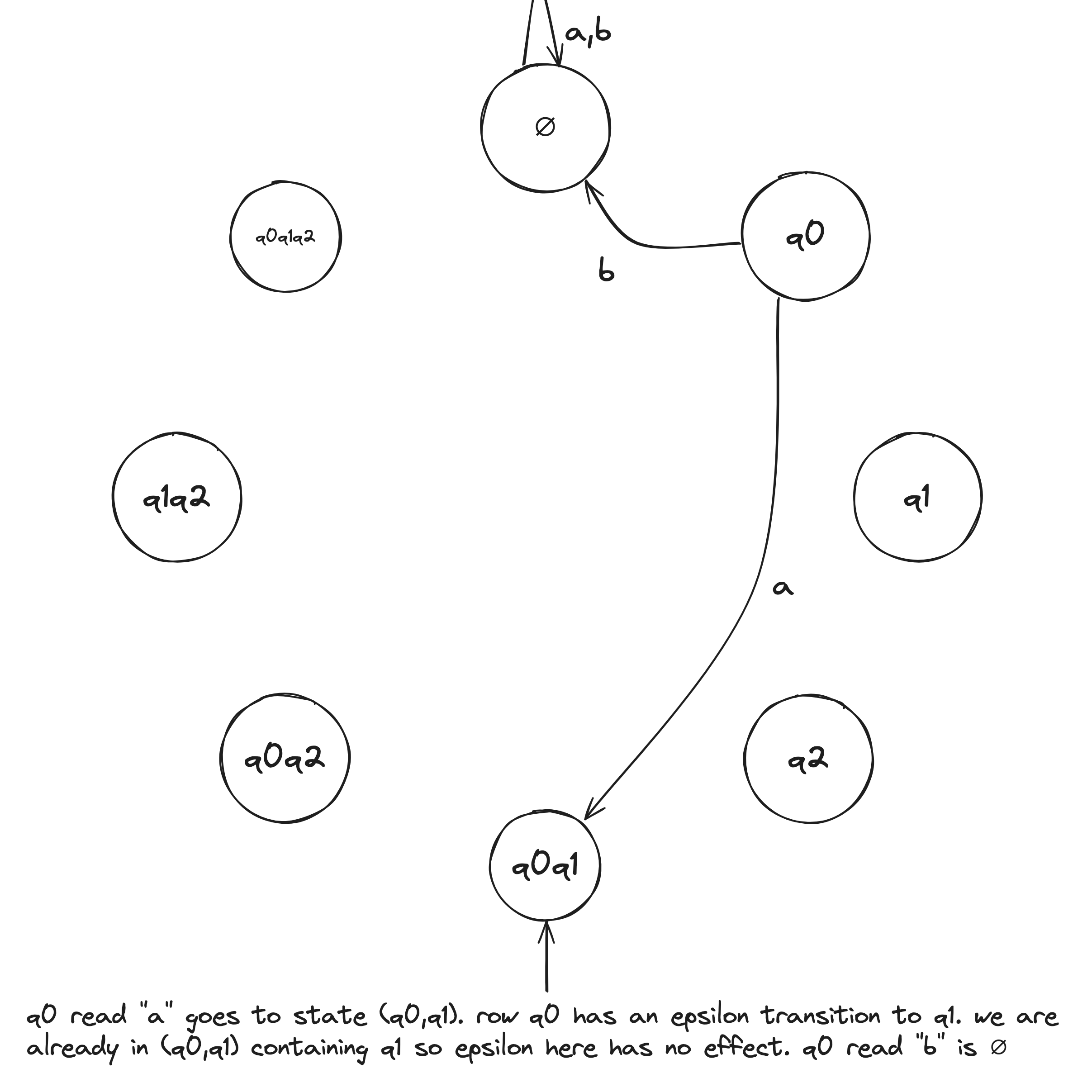
- Draw transitions whereafter the first transition, look to the epsilon column and, if it's not an empty set (epsilon column entry), include it in the tuple.
- Define accepting states to be the states containing .
Regular Expressions
is a regular expression if is
- for some in the alphabet
- , representing the language containing a single string—the empty string
- , representing the language containing no strings
- where and are regular expressions
- where and are regular expressions
- where is a regular expression
Regex Examples
Given , in the format :
- contains a single 1: , star means zero or more
- has at least one 1: , means any symbol in the alphabet
- contains the substring 001:
- every 0 in is followed by at least one 1: , plus means one or more
- is a string of even length: , a string of 0 length is even
- the length of is a multiple of 3:
- the language :
- starts and ends with the same symbol:
- , describes , and the concatenation adds either 0 or before every string in
- , it's kind of like the FOIL method
- , concatenating the empty set to any set yields the empty set
Let be any expression, we have the following identities:
- , adding the empty language to any other language will not change it
- , joining any string to the empty string will not change it
- may not equal , e.g., if , then but
- may not equal , e.g., if , then but
Regex to NFA
Let regular expression describe some language .
Convert into an NFA recognizing .
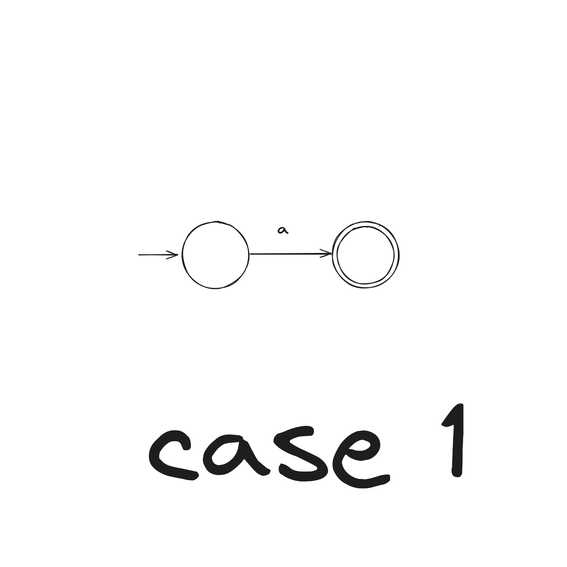
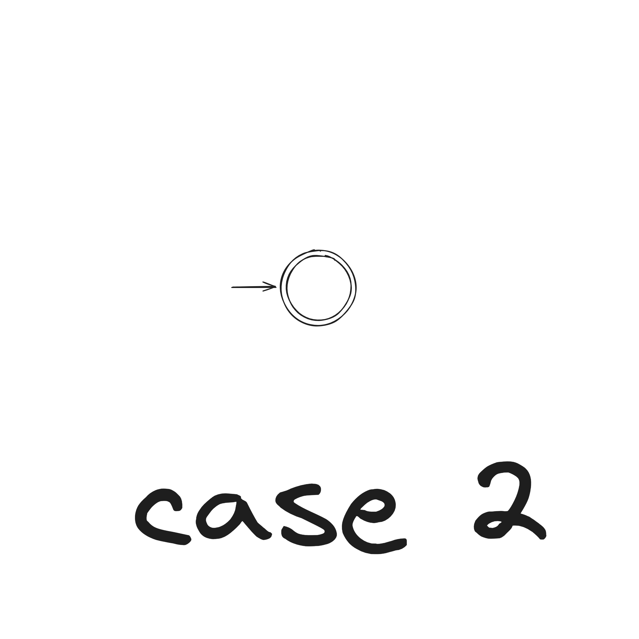
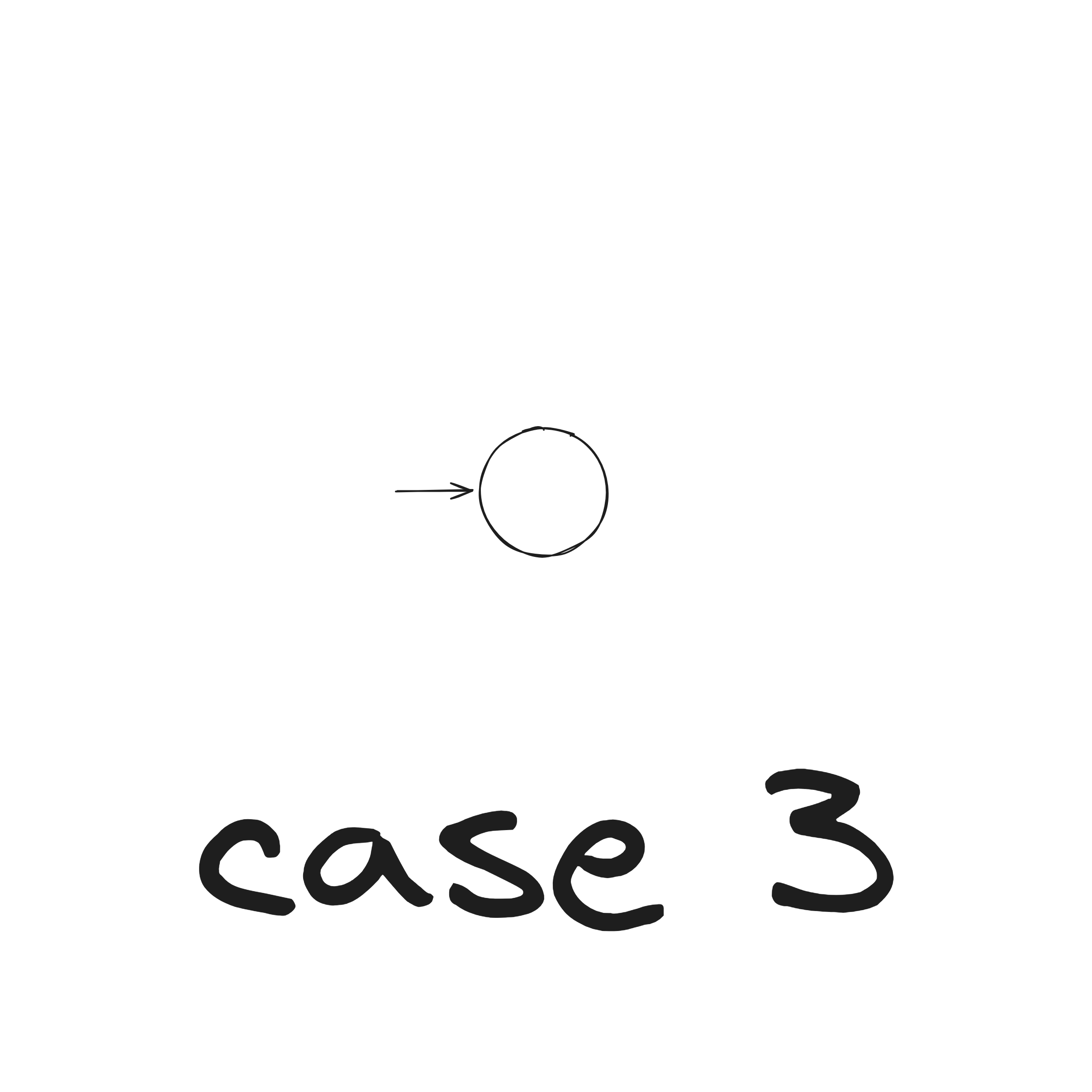
There are six cases:
- , see nondeterministic version of the union operation proof
- , see concatenation operation proof
- , see kleene star operation proof
DFA to Regex
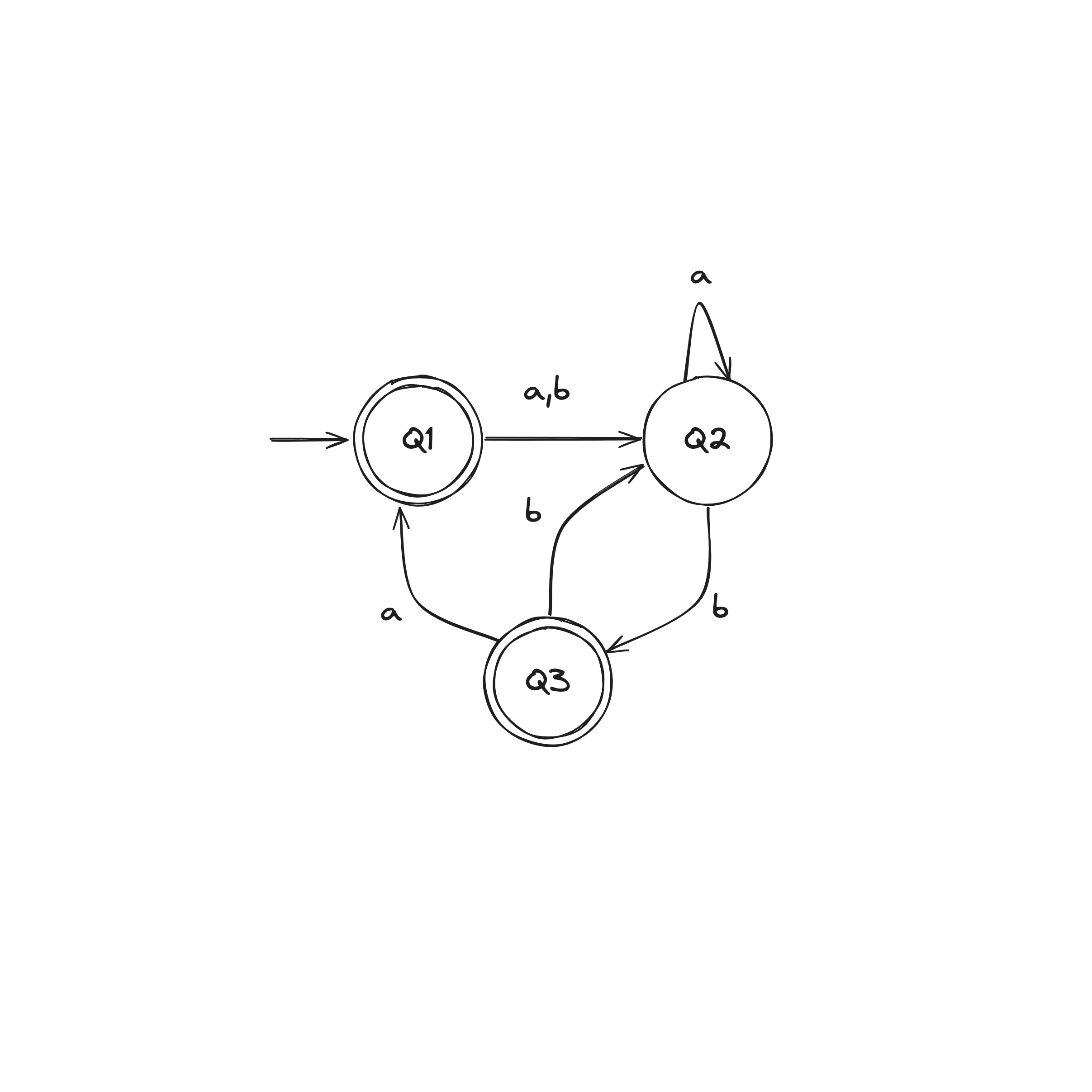
Let a DFA recognize a language .
Convert the DFA into equivalent regular expressions in following steps:
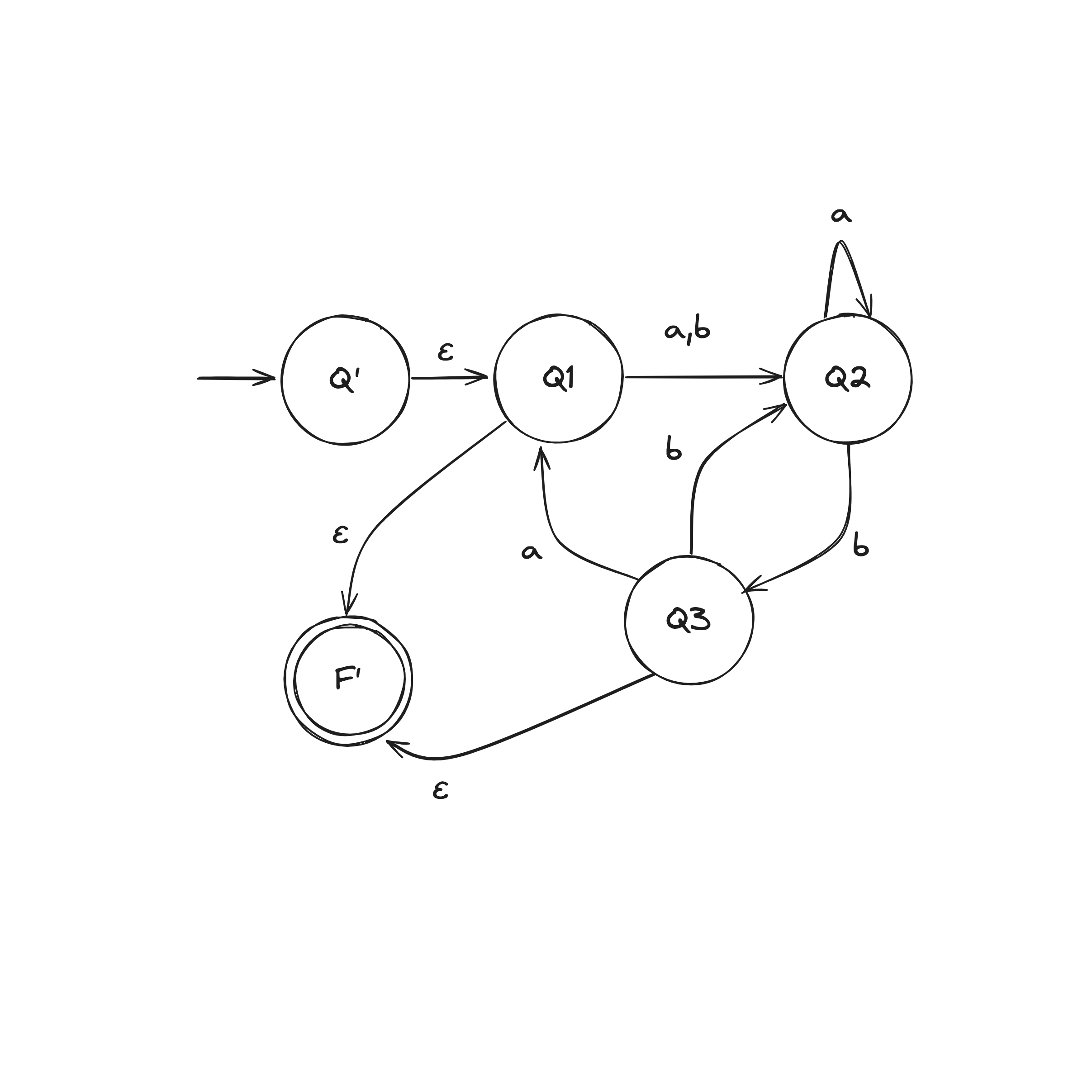
Step 1. Convert DFA into a GNFA (generalized nondeterministic finite automaton)
Let DFA recognize .
We construct GNFA :
- remains the same
- is the new start state
- Define so that for any and any :
This construction does not explicitly redefine the transitions into regular expressions over . We just do that in our heads.
Step 2. Convert GNFA into regular expressions
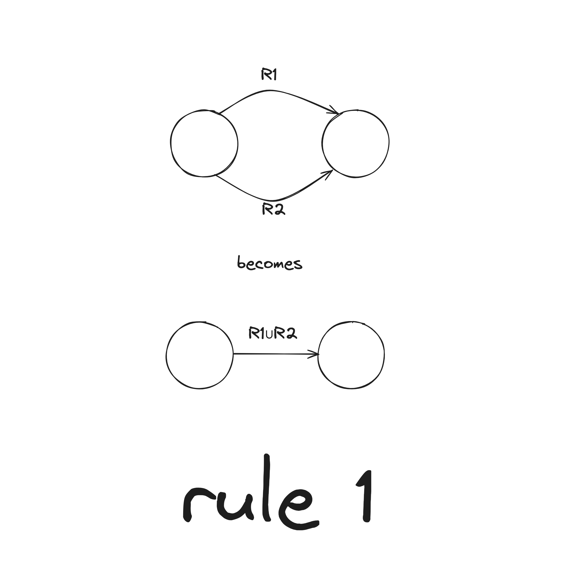
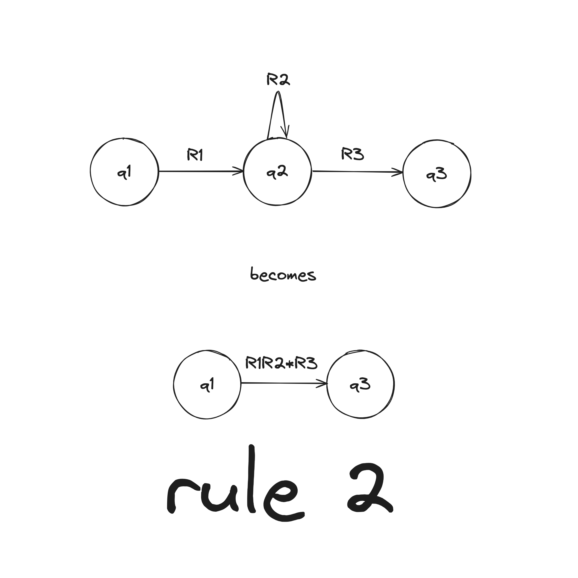
There are two rules when collapsing a GNFA into a 2-state:
DFA to Regex Example
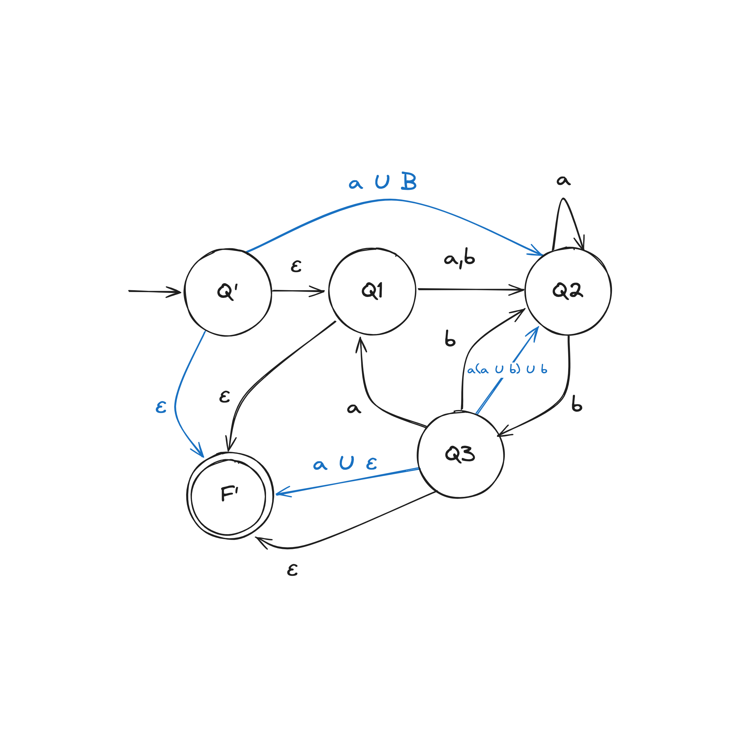
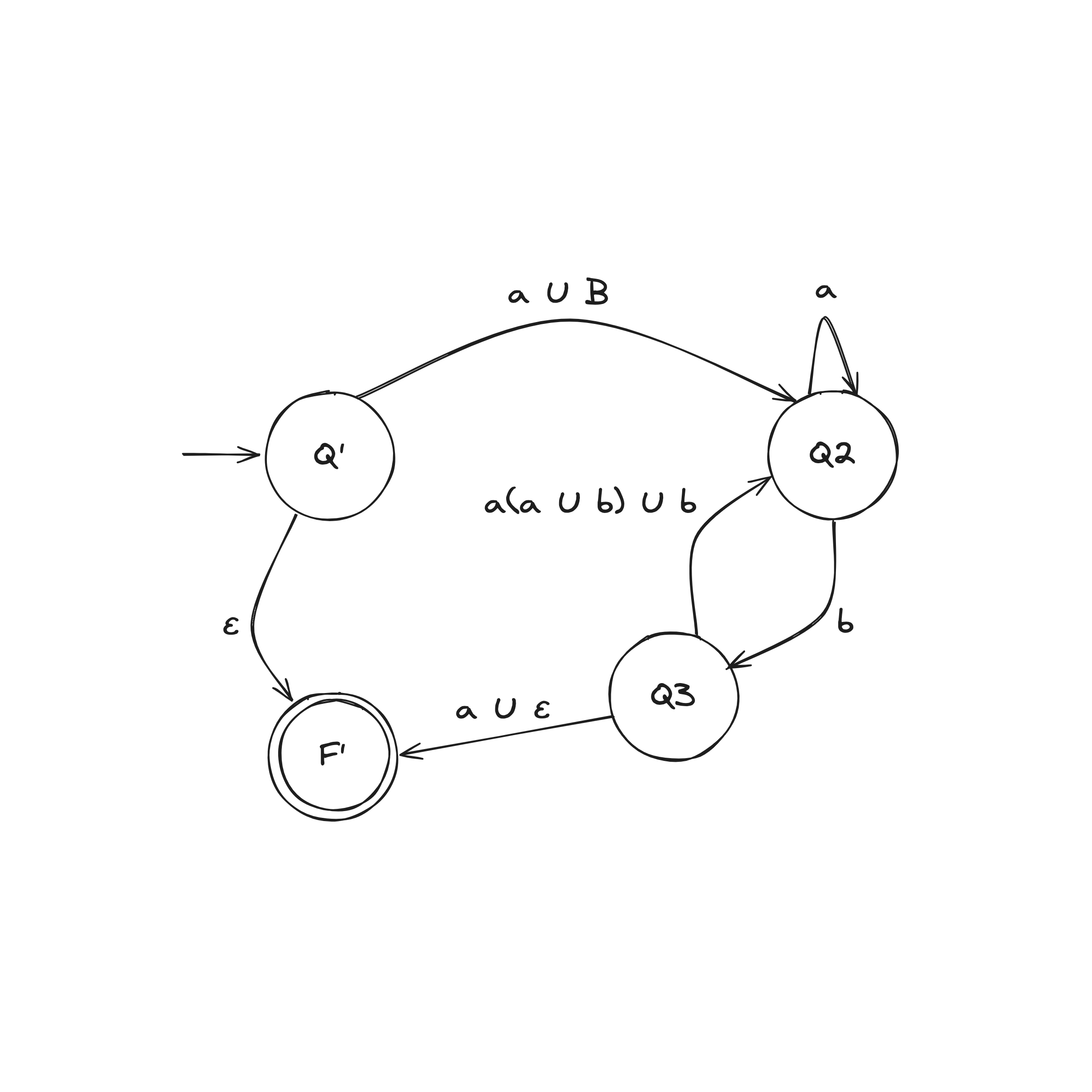
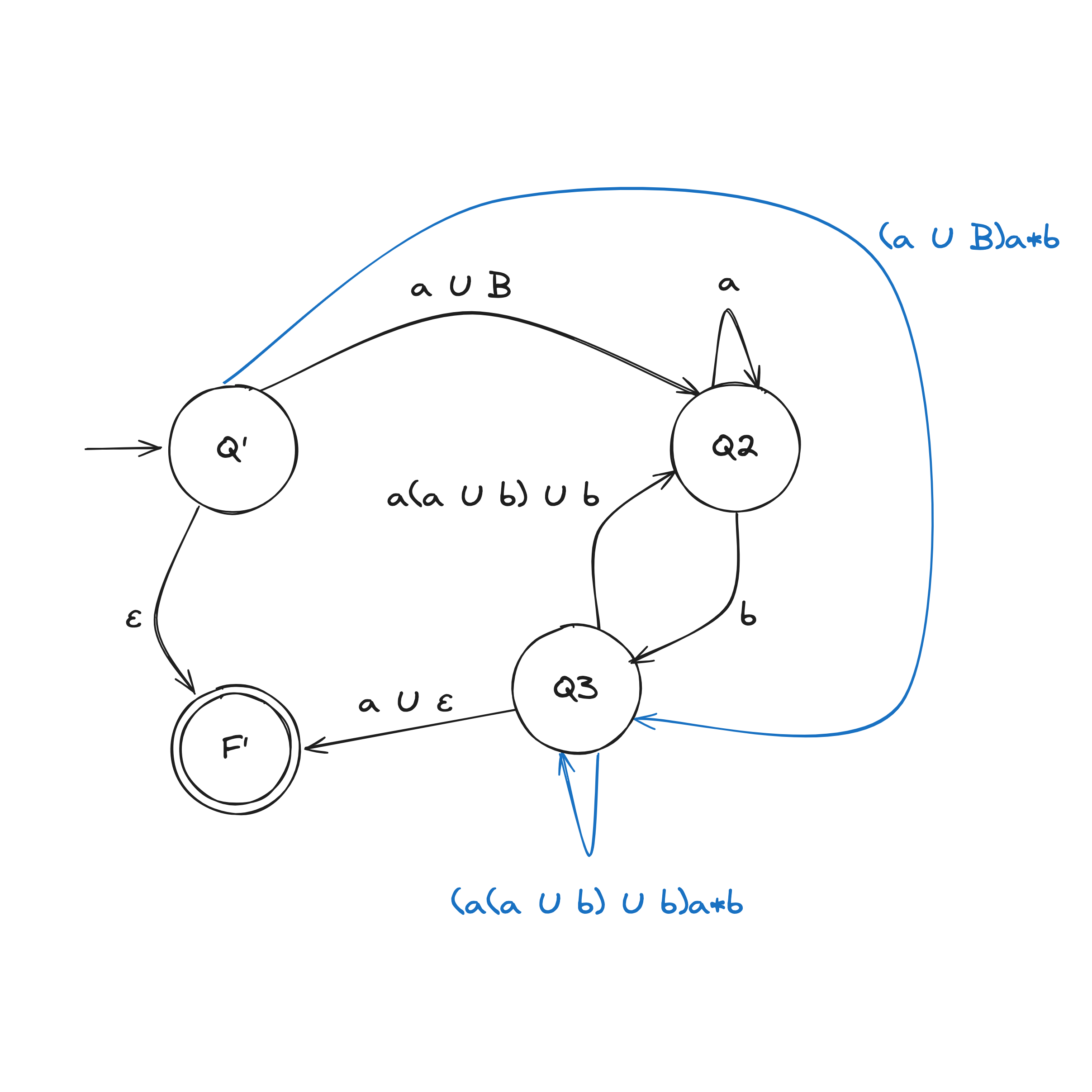
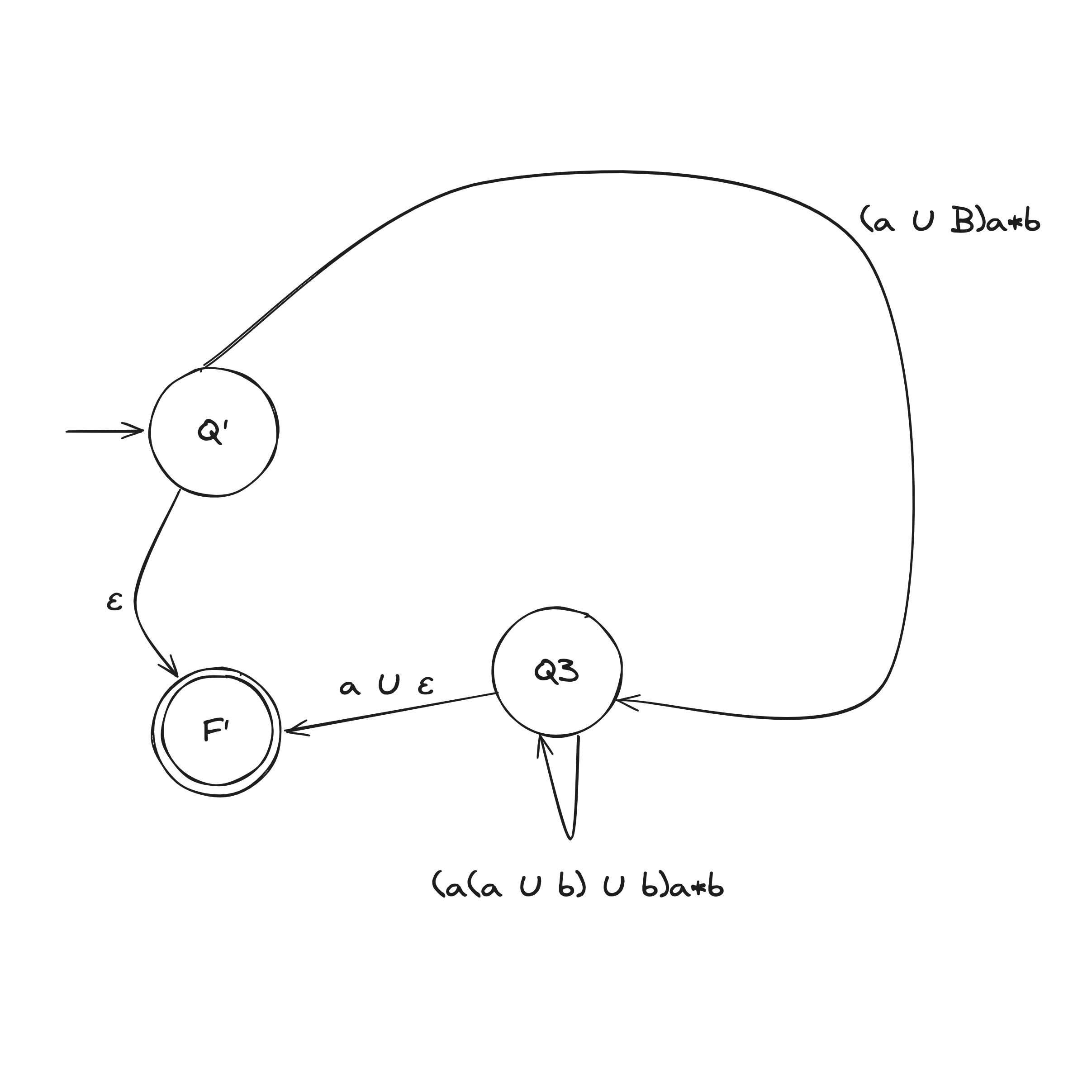
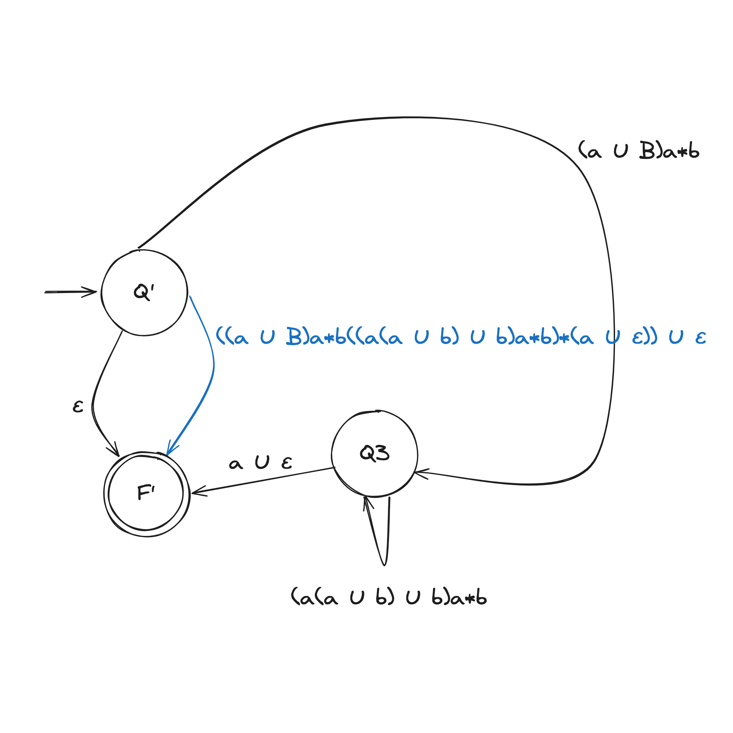
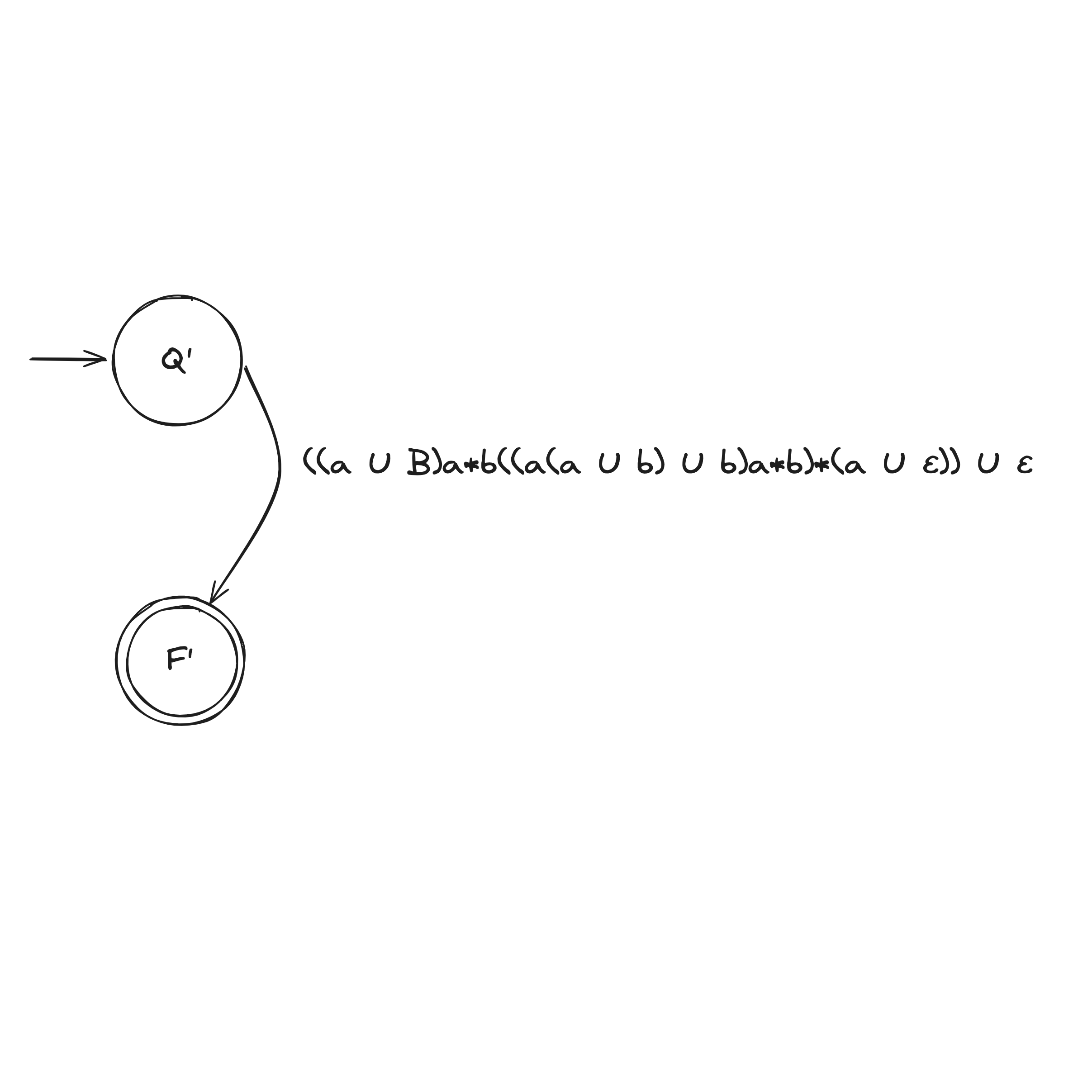
Computability Theory
The main objective of computability theory is to classify problems as solvable or unsolvable
Complexity Theory
The main objective of complexity theory is to classify problems as easy or hard.
An important question capturing this idea:
What makes some problems computationally hard and others easy?